setwd("C:/Users/devmbeya/Documents/giswithrtutorials")
getwd() #check the file path of the current directory
[1] "C:/Users/devmbeya/Documents/giswithrtutorials"In this tutorial, you will learn how to select geographic features based on their association with non-spatial and also based on their location.
Set working directory
setwd("C:/Users/devmbeya/Documents/giswithrtutorials")
getwd() #check the file path of the current directory[1] "C:/Users/devmbeya/Documents/giswithrtutorials"Load required packages
library(sf)
library(dplyr)
Read data
africa <- st_read("../assets/data/vector/africa.shp")Reading layer `africa' from data source
`C:\Users\devmbeya\Downloads\gis-remote-sensing-r\assets\data\vector\africa.shp'
using driver `ESRI Shapefile'
Simple feature collection with 55 features and 13 fields
Geometry type: MULTIPOLYGON
Dimension: XY
Bounding box: xmin: -25.36042 ymin: -46.96575 xmax: 51.41704 ymax: 37.3452
Geodetic CRS: WGS 84africa_project <- st_read("../assets/data/vector/africa_project.shp")Reading layer `africa_project' from data source
`C:\Users\devmbeya\Downloads\gis-remote-sensing-r\assets\data\vector\africa_project.shp'
using driver `ESRI Shapefile'
Simple feature collection with 55 features and 15 fields
Geometry type: MULTIPOLYGON
Dimension: XY
Bounding box: xmin: -4296552 ymin: -3854841 xmax: 3987157 ymax: 4134822
Projected CRS: Africa_Sinusoidalafrica_continent <- st_read("../assets/data/vector/africa_continent.shp")Reading layer `africa_continent' from data source
`C:\Users\devmbeya\Downloads\gis-remote-sensing-r\assets\data\vector\africa_continent.shp'
using driver `ESRI Shapefile'
Simple feature collection with 1 feature and 6 fields
Geometry type: MULTIPOLYGON
Dimension: XY
Bounding box: xmin: -25.36055 ymin: -34.822 xmax: 63.49576 ymax: 37.34041
Geodetic CRS: WGS 84cities <- st_read("../assets/data/vector/africa_capital_cities.shp")Reading layer `africa_capital_cities' from data source
`C:\Users\devmbeya\Downloads\gis-remote-sensing-r\assets\data\vector\africa_capital_cities.shp'
using driver `ESRI Shapefile'
Simple feature collection with 51 features and 14 fields
Geometry type: POINT
Dimension: XY
Bounding box: xmin: -23.521 ymin: -29.308 xmax: 47.528 ymax: 36.819
Geodetic CRS: WGS 84roads <- st_read("../assets/data/vector/africa_roads.shp")Reading layer `africa_roads' from data source
`C:\Users\devmbeya\Downloads\gis-remote-sensing-r\assets\data\vector\africa_roads.shp'
using driver `ESRI Shapefile'
Simple feature collection with 2581 features and 30 fields
Geometry type: MULTILINESTRING
Dimension: XY
Bounding box: xmin: -17.45546 ymin: -34.2343 xmax: 49.41792 ymax: 37.10583
Geodetic CRS: WGS 84GIS data comes in two forms: spatial and attribute data. Spatial data represents the aspects of geography inform of map layers. Attribute data in GIS describe the properties or characteristics of the spatial features. A school would have its spatial data represented as geographic coordinates(latitudes and longitudes) and its attribute data would include name of the school, student enrollment, number of teachers, name of district it is located in etc.
Attribute queries select geographic features based on their association with attributes (non-spatial data). This is achieved by using conditions such as field names(e.g., ADIMN, NAME), operators (e.g., <, >, =, ==) and values (e.g., Malawi, TRUE, 20000).
Simple feature collection with 55 features and 13 fields
Geometry type: MULTIPOLYGON
Dimension:     XY
Bounding box:  xmin: -25.36042 ymin: -46.96575 xmax: 51.41704 ymax: 37.3452
Geodetic CRS:  WGS 84
First 10 features:
                         ADMIN ADM0_A3   POP_EST POP_RANK POP_YEAR GDP_MD
1                     Ethiopia     ETH 112078730       17     2019  95912
2                  South Sudan     SDS  11062113       14     2019  11998
3                      Somalia     SOM  10192317       14     2019   4719
4                        Kenya     KEN  52573973       16     2019  95503
5                       Malawi     MWI  18628747       14     2019   7666
6  United Republic of Tanzania     TZA  58005463       16     2019  63177
7                   Somaliland     SOL   5096159       13     2014  17836
8                      Morocco     MAR  36471769       15     2019 119700
9               Western Sahara     SAH    603253       11     2017    907
10       Republic of the Congo     COG   5380508       13     2019  12267
   GDP_YEAR                   ECONOMY             INCOME_GRP CONTINENT
1      2019 7. Least developed region          5. Low income    Africa
2      2015 7. Least developed region          5. Low income    Africa
3      2016 7. Least developed region          5. Low income    Africa
4      2019   5. Emerging region: G20          5. Low income    Africa
5      2019 7. Least developed region          5. Low income    Africa
6      2019 7. Least developed region          5. Low income    Africa
7      2013      6. Developing region 4. Lower middle income    Africa
8      2019      6. Developing region 4. Lower middle income    Africa
9      2007 7. Least developed region          5. Low income    Africa
10     2019      6. Developing region 4. Lower middle income    Africa
         SUBREGION                  REGION_WB               NAME_EN
1   Eastern Africa         Sub-Saharan Africa              Ethiopia
2   Eastern Africa         Sub-Saharan Africa           South Sudan
3   Eastern Africa         Sub-Saharan Africa               Somalia
4   Eastern Africa         Sub-Saharan Africa                 Kenya
5   Eastern Africa         Sub-Saharan Africa                Malawi
6   Eastern Africa         Sub-Saharan Africa              Tanzania
7   Eastern Africa         Sub-Saharan Africa            Somaliland
8  Northern Africa Middle East & North Africa               Morocco
9  Northern Africa Middle East & North Africa        Western Sahara
10   Middle Africa         Sub-Saharan Africa Republic of the Congo
                         geometry
1  MULTIPOLYGON (((34.0707 9.4...
2  MULTIPOLYGON (((35.92084 4....
3  MULTIPOLYGON (((46.46696 6....
4  MULTIPOLYGON (((35.70585 4....
5  MULTIPOLYGON (((34.96461 -1...
6  MULTIPOLYGON (((32.92086 -9...
7  MULTIPOLYGON (((48.93911 11...
8  MULTIPOLYGON (((-8.817035 2...
9  MULTIPOLYGON (((-8.817035 2...
10 MULTIPOLYGON (((18.62639 3.... [1] "ADMIN" "ADM0_A3" "POP_EST" "POP_RANK" "POP_YEAR"
[6] "GDP_MD" "GDP_YEAR" "ECONOMY" "INCOME_GRP" "CONTINENT"
[11] "SUBREGION" "REGION_WB" "NAME_EN" "geometry" Geometry set for 55 features
Geometry type: MULTIPOLYGON
Dimension: XY
Bounding box: xmin: -25.36042 ymin: -46.96575 xmax: 51.41704 ymax: 37.3452
Geodetic CRS: WGS 84
First 5 geometries: [1] "Ethiopia" "South Sudan"
[3] "Somalia" "Kenya"
[5] "Malawi" "United Republic of Tanzania"
[7] "Somaliland" "Morocco"
[9] "Western Sahara" "Republic of the Congo"
[11] "Democratic Republic of the Congo" "Namibia"
[13] "South Africa" "Libya"
[15] "Tunisia" "Zambia"
[17] "Sierra Leone" "Guinea"
[19] "Liberia" "Central African Republic"
[21] "Sudan" "Djibouti"
[23] "Eritrea" "Ivory Coast"
[25] "Mali" "Senegal"
[27] "Nigeria" "Benin"
[29] "Angola" "Botswana"
[31] "Zimbabwe" "Chad"
[33] "Algeria" "Mozambique"
[35] "eSwatini" "Burundi"
[37] "Rwanda" "Uganda"
[39] "Lesotho" "Cameroon"
[41] "Gabon" "Niger"
[43] "Burkina Faso" "Togo"
[45] "Ghana" "Guinea-Bissau"
[47] "Egypt" "Mauritania"
[49] "Equatorial Guinea" "Gambia"
[51] "Bir Tawil" "Madagascar"
[53] "Comoros" "São Tomé and Principe"
[55] "Cabo Verde" In R, you van use dplyr subsetting functions to select a subset of the data: rows or columns. You can use the filter() and slice functions to select rows and select() to subset columns.
Select countries with population greater than 80 million. Use the dplyr’s filter() function.
# Once again explore the data
head(africa)
Simple feature collection with 6 features and 13 fields
Geometry type: MULTIPOLYGON
Dimension: XY
Bounding box: xmin: 24.12156 ymin: -17.13534 xmax: 51.41704 ymax: 14.87953
Geodetic CRS: WGS 84
ADMIN ADM0_A3 POP_EST POP_RANK POP_YEAR GDP_MD
1 Ethiopia ETH 112078730 17 2019 95912
2 South Sudan SDS 11062113 14 2019 11998
3 Somalia SOM 10192317 14 2019 4719
4 Kenya KEN 52573973 16 2019 95503
5 Malawi MWI 18628747 14 2019 7666
6 United Republic of Tanzania TZA 58005463 16 2019 63177
GDP_YEAR ECONOMY INCOME_GRP CONTINENT SUBREGION
1 2019 7. Least developed region 5. Low income Africa Eastern Africa
2 2015 7. Least developed region 5. Low income Africa Eastern Africa
3 2016 7. Least developed region 5. Low income Africa Eastern Africa
4 2019 5. Emerging region: G20 5. Low income Africa Eastern Africa
5 2019 7. Least developed region 5. Low income Africa Eastern Africa
6 2019 7. Least developed region 5. Low income Africa Eastern Africa
REGION_WB NAME_EN geometry
1 Sub-Saharan Africa Ethiopia MULTIPOLYGON (((34.0707 9.4...
2 Sub-Saharan Africa South Sudan MULTIPOLYGON (((35.92084 4....
3 Sub-Saharan Africa Somalia MULTIPOLYGON (((46.46696 6....
4 Sub-Saharan Africa Kenya MULTIPOLYGON (((35.70585 4....
5 Sub-Saharan Africa Malawi MULTIPOLYGON (((34.96461 -1...
6 Sub-Saharan Africa Tanzania MULTIPOLYGON (((32.92086 -9...# Select countries with population greater than 80 million
pop <- filter(africa, POP_EST > 80000000)
popSimple feature collection with 4 features and 13 fields
Geometry type: MULTIPOLYGON
Dimension: XY
Bounding box: xmin: 2.671082 ymin: -13.45835 xmax: 47.97917 ymax: 31.65648
Geodetic CRS: WGS 84
ADMIN ADM0_A3 POP_EST POP_RANK POP_YEAR GDP_MD
1 Ethiopia ETH 112078730 17 2019 95912
2 Democratic Republic of the Congo COD 86790567 16 2019 50400
3 Nigeria NGA 200963599 17 2019 448120
4 Egypt EGY 100388073 17 2019 303092
GDP_YEAR ECONOMY INCOME_GRP CONTINENT
1 2019 7. Least developed region 5. Low income Africa
2 2019 7. Least developed region 5. Low income Africa
3 2019 5. Emerging region: G20 4. Lower middle income Africa
4 2019 5. Emerging region: G20 4. Lower middle income Africa
SUBREGION REGION_WB NAME_EN
1 Eastern Africa Sub-Saharan Africa Ethiopia
2 Middle Africa Sub-Saharan Africa Democratic Republic of the Congo
3 Western Africa Sub-Saharan Africa Nigeria
4 Northern Africa Middle East & North Africa Egypt
geometry
1 MULTIPOLYGON (((34.0707 9.4...
2 MULTIPOLYGON (((18.62639 3....
3 MULTIPOLYGON (((3.5964 11.6...
4 MULTIPOLYGON (((34.24835 31...# Plot the selected polygons
plot(pop$geometry)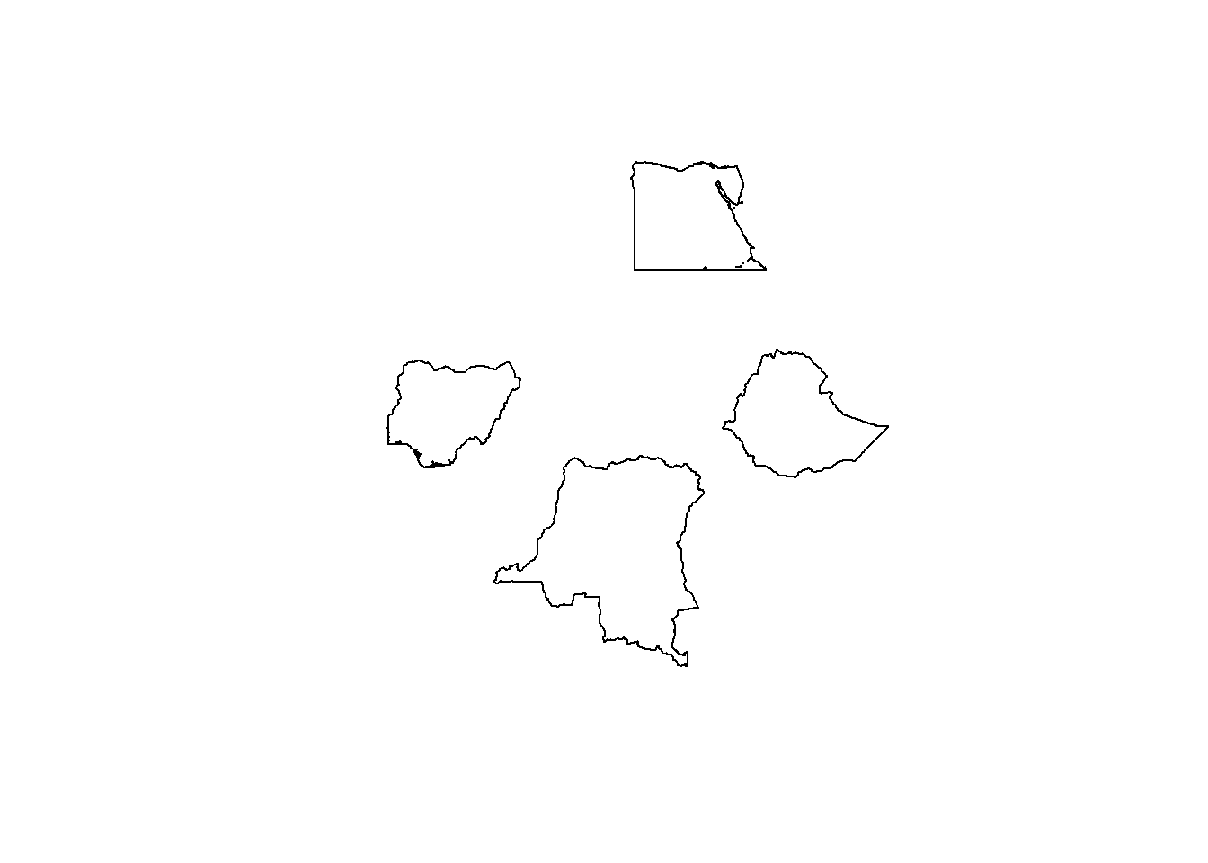
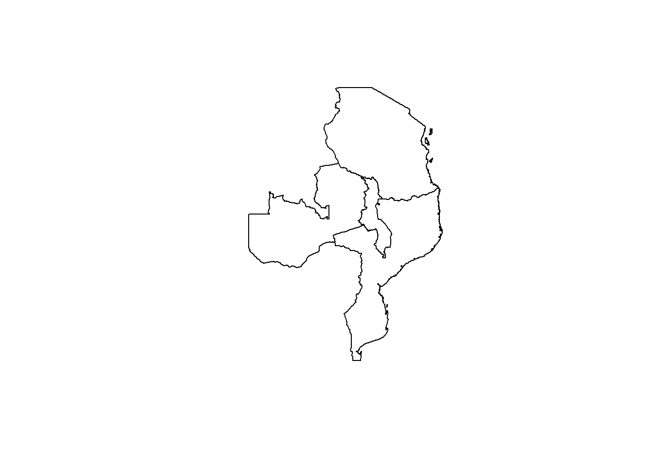
Select South Africa and Malawi polygons
south_africa <- filter(africa, NAME_EN == 'South Africa' | NAME_EN=="Malawi")

plot(south_africa$geometry)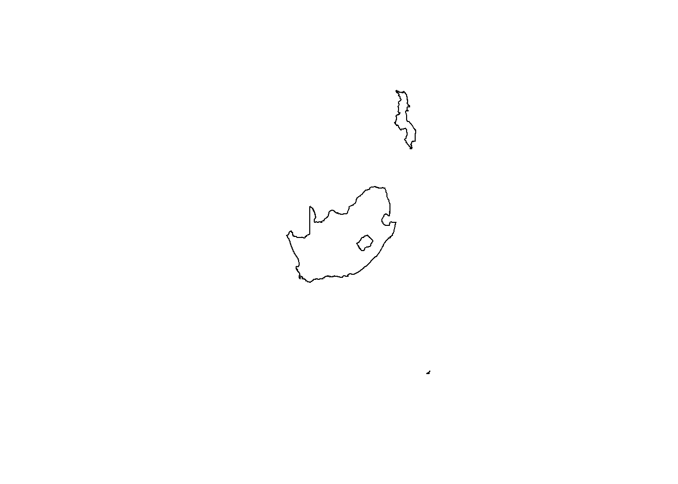
Select Malawi’s neighbors
To select features by their location, we can use topological relations between vector geometries.
To select features by their location, we can use topological relations between vector geometries in sf. Common functions include:
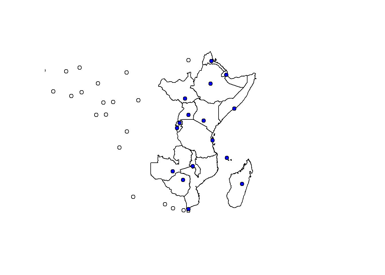
st_intersects(x, y) – returns features in x that intersect features in y.st_touches(x, y) – returns features in x that touch features in y (share a boundary but do not overlap).st_overlaps(x, y) – returns features in x that overlap features in y partially.st_contains(x, y) – returns features in x that contain features in y.st_contains_properly(x, y) – stricter version of st_contains.st_covers(x, y) – returns features in x that cover features in y.st_within(x, y) – returns features in x that are within features in y.st_covered_by(x, y) – returns features in x that are covered by features in y.st_disjoint(x, y) – returns features in x that do not intersect features in y.Select cities that are located within East African countries.
# Select countries within Eastern Africa
east_africa <- filter(africa, SUBREGION == 'Eastern Africa')

# Plot East African countries
plot(east_africa$geometry)

# Select and plot all eastern African cities
east_cities <- st_intersection(x = cities, y=east_africa)

plot(east_cities$geometry, add=TRUE, col='blue', pch=16)

plot(cities$geometry, add=TRUE)