#setwd("C:/Users/devmbeya/Documents/rtutorials")
# Change C:/Users/devmbeya/Documents/rmentorshipprogram/cohort1 path to your working directoryR basics
Introduction to R
In this tutorial, we lay the foundation for working with R by exploring its core concepts and essential tools. Our focus is on building a strong understanding of the R environment and basic operations that will support advanced geospatial and remote sensing tasks in later tutorials. Specifically, we cover how to set up a working directory, install and load packages, create and manage variables, and understand R data types and data structures. We also introduce R functions, demonstrate how to create basic plots for data visualization.
What you will learn:
- Understand the R environment and set up a working directory.
- Learn how to install and load packages for extended functionality.
- Explore variable creation, data types, and data structures in R.
- Gain familiarity with writing and using functions in R.
- Create simple plots for basic data visualization.
What is R?
R is a popular programming language used for statistical computing and graphical presentation.
Why use R?
- It is a great resource for data analysis, data visualization, data science and machine learning
- It provides many statistical techniques (such as statistical tests, classification, clustering and data reduction)
- It is easy to draw graphs in R, like pie charts, histograms, box plot, scatter plot, etc++
- It works on different platforms (Windows, Mac, Linux)
- It is open-source and free
- It has a large community support
- It has many packages (libraries of functions) that can be used to solve different problems
Setting working directory
A working directory in R is a specific location (a folder or directory) on your computer that R uses as the default place to look for files when you try to read them into R, and where it will save files when you write them out from R. To set a working directory in we use the setwd("path to your directory") function.
The code above sets rtutorials folder located in the Documents library as a working directory.
R Variables
Variables are containers for storing data values. R does not have a command for declaring a variable. A variable is created the moment you first assign a value.
x <- 2  # assigns a value 2 to a variable x

x = 2  # assigns a value 2 to a variable x

assign('x', 2) # assigns a value 2 to a variable x

x # print a value stored in x
[1] 2print(x) # print a value stored in x[1] 2Using an = variable assignment operator is discouraged because it can cause errors in some cases. It is not necessary to use print() function unless you are working with loops.
Try it yourself
Create a variable named height with value 175, and weight with value 68.Then print both.
# Your code here:Basic R data types
R has the following types:
- numeric: (10.5, 55, 787)
- integer: (1L, 55L, 100L, where the letter “L” declares this as an integer)
- complex: (9 + 3i, where “i” is the imaginary part)
- character (a.k.a. string): (“k”, “R is exciting”, “FALSE”, “11.5”)
- logical (a.k.a. boollean): (TRUE or FALSE)
my_numeric <- 12.5    #my_numeric is a numeric variable

my_numeric  # print my_numeric value
[1] 12.5my_logical <- TRUE # my_logical is a logical(Boolean) variable
my_logical # Display my_logical value[1] TRUEcountry <- "Angola" # Country is a character variable
country[1] "Angola"Characters(string or text) are closed in single(’’) or double quotes(““)
country <- "10"
country   # country is still character
[1] "10"To check the data type use the class() function.
class(my_numeric) # check the type of a variable [1] "numeric"class(country)[1] "character"Try it yourself
- Create a numeric variable
xwith value3.14. - Create a character variable
ywith valueR is fun - Create a logical variable
zwith valueTRUE.
# Your code here:R functions
A function is a block of organized, reusable code that performs a specific task. Functions are fundamental to R programming, enabling modularity, code reusability, and easier problem-solving.
R provides a comprehensive set of built-in functions for various tasks, including mathematical operations, statistical analysis, data manipulation, and input/output. These functions are pre-defined and can be directly utilized without requiring the user to write the underlying code.
Built-in Function are the functions that are already existing in R language and we just need to call them to use.
Examples of built in functions: * C(): combine function which combines valuesinto a vector * sum(): adds values * max(): returns maximum value * min(): returns the minimun value * seq(1:10): creates a seqiuence of numbers
x <- c(1,2,3)

sum(x)
[1] 6max(x) [1] 3min(x) [1] 1R packages
R packages are a collection of R functions compiled code and sample data R packages are stored under a directory called ‘library’ in the R environment Packages need to be installed before they can be used in R. Packages are installed using install.packages(“package name”)
#install.packages("sf") #Installs the simple feature, sf, package.
#library()     #gets the list of installed packages
When a package has been installed, it has to be loaded/imported into R for it to be used. Packages are loaded using library(package name)
library(sf)R data structures
A data structure is a particular way of organizing data in a computer so that it can be used effectively. The idea is to reduce the space and time complexities of different tasks. Data structures in R programming are tools for holding multiple values. R has six data structures:
1. Vectors
A vector is an ordered collection of basic data types of a given length. The only key thing here is all the elements of a vector must be of the identical data type e.g homogeneous data structures. Vectors are one-dimensional data structures.
x <- c(1, 2, 3, 4, 5)
x
[1] 1 2 3 4 52. Lists
A list is a generic object consisting of an ordered collection of objects. Lists are heterogeneous data structures. These are also one-dimensional data structures. A list can be a list of vectors, list of matrices, a list of characters and a list of functions and so on.
studentName <- c("James", "John", "Mercy")
studentID <- c(2020, 2030, 2040)
yearOfStudy <- c(1, 2, 2)

mylist <- list(studentName, studentID, yearOfStudy)
mylist
[[1]]
[1] "James" "John" "Mercy"
[[2]]
[1] 2020 2030 2040
[[3]]
[1] 1 2 2Try it yourself
- Create a vector
agescontaining 18, 25, 30, 45. - Create a list
personwith “name=Alice”, “age=25” and “is_student=TRUE”.
# Your code here:3. Data frame
Data frames are generic data objects of R which are used to store the tabular data. Data frames are the foremost popular data objects in R programming because we are comfortable in seeing the data within the tabular form. They are two-dimensional, heterogeneous data structures. These are lists of vectors of equal lengths.
Data frames have the following constraints placed upon them:
- A data-frame must have column names and every row should have a unique name.
- Each column must have the identical number of items.
- Each item in a single column must be of the same data type.
- Different columns may have different data types.
- To create a data frame we use the data.frame() function.
- R data structures: vector, matrix, list, data frame
studentName <- c("James", "John", "Mercy")
studentID <- c(2020, 2030, 2040)
yearOfStudy <- c(1, 2, 2)

myDataframe <- data.frame(studentName, studentID, yearOfStudy)
myDataframe
studentName studentID yearOfStudy
1 James 2020 1
2 John 2030 2
3 Mercy 2040 2Try it yourself
Create a data frame called “students” with two columns: “name = c(”John”, “Jane”, “Mike”)“,”score = c(85, 90, 78)“. Print the data frame.
# Your code here:4. Matrices
A matrix is a rectangular arrangement of numbers in rows and columns. In a matrix, as we know rows are the ones that run horizontally and columns are the ones that run vertically. Matrices are two-dimensional, homogeneous data structures.
y <- matrix (
  c(10, 20, 30, 40, 50, 60, 70, 80, 90, 100),
  nrow = 3, ncol = 3,
  byrow = TRUE
)

y
[,1] [,2] [,3]
[1,] 10 20 30
[2,] 40 50 60
[3,] 70 80 905. Arrays
Arrays are the R data objects which store the data in more than two dimensions. Arrays are n-dimensional data structures. For example, if we create an array of dimensions (2, 3, 3) then it creates 3 rectangular matrices each with 2 rows and 3 columns. They are homogeneous data structures.
myArray <- array(
  c(10, 20, 30, 40, 50, 60, 70, 80, 90, 100),
  dim = c(2, 2, 2)
)

myArray
, , 1
[,1] [,2]
[1,] 10 30
[2,] 20 40
, , 2
[,1] [,2]
[1,] 50 70
[2,] 60 806. Factors
Factors are the data objects which are used to categorize the data and store it as levels. They are useful for storing categorical data. They can store both strings and integers. They are useful to categorize unique values in columns like (“TRUE” or “FALSE”) or (“MALE” or “FEMALE”), etc..
They are useful in data analysis for statistical modeling.
myFactor <- factor(c("male", "female", "male", "female"))
myFactor
[1] male female male female
Levels: female maleData structures example
Imagine that one you are analyzing weather data (amount of rainfall and the magnitude of temperature) recorded at a particular weather station from Monday, 16th March 2024 to Saturday, 21st March 2024. The observations recorded are as follows:
Rainfall readings in mm
- Monday March 16 2024: 10
- Tuesday March 17 2024: 20
- Wednesday March 18 2024: 11
- Thursday March 19 2024: 30
- Friday March 20 2024: 15
- Saturday March 21 2024: 9
- Sunday March 22 2024:10
Temperature readings in degrees Celsius
- Monday March 16 2024: 16
- Tuesday March 17 2024: 17
- Wednesday March 18 2024: 25
- Thursday March 19 2024: 23
- Friday March 20 2024: 17
- Saturday March 21 2024: 27
- Sunday March 22 2024: 13
Step one
To work with this data in R, firstly create the vectors Rainfall, Temperature and Date
rainfall <- c(10, 20, 11, 30, 15, 9, 10)

max(rainfall)
[1] 30min(rainfall)[1] 9temperature <- c(16, 17, 25, 23, 17, 27, 13)
temperature[1] 16 17 25 23 17 27 13min(temperature)[1] 13day <- c("Monday", "Tuesday", "Wednesday", "Thursday", "Friday", "Saturday", "Sunday")
day[1] "Monday" "Tuesday" "Wednesday" "Thursday" "Friday" "Saturday"
[7] "Sunday" date <- as.Date(c("2024-03-16", "2024-03-17", "2024-03-18", "2024-03-19", "2024-03-20", "2024-03-21", "2024-03-22"))
date[1] "2024-03-16" "2024-03-17" "2024-03-18" "2024-03-19" "2024-03-20"
[6] "2024-03-21" "2024-03-22"class(date)[1] "Date"Present the data in a Data Frame
myweather <- data.frame(day,
                        date,
                        rainfall,
                        temperature
                       )
myweather
day date rainfall temperature
1 Monday 2024-03-16 10 16
2 Tuesday 2024-03-17 20 17
3 Wednesday 2024-03-18 11 25
4 Thursday 2024-03-19 30 23
5 Friday 2024-03-20 15 17
6 Saturday 2024-03-21 9 27
7 Sunday 2024-03-22 10 13head(myweather) #shows first 6 rows day date rainfall temperature
1 Monday 2024-03-16 10 16
2 Tuesday 2024-03-17 20 17
3 Wednesday 2024-03-18 11 25
4 Thursday 2024-03-19 30 23
5 Friday 2024-03-20 15 17
6 Saturday 2024-03-21 9 27head(myweather, 3) #shows first 3 rows day date rainfall temperature
1 Monday 2024-03-16 10 16
2 Tuesday 2024-03-17 20 17
3 Wednesday 2024-03-18 11 25# Sub-setting a data frame
myweather[1, 2] # returns the data frame element for the first row and second column[1] "2024-03-16"myweather[ ,1] # returns data frame elements for first column and all rows[1] "Monday" "Tuesday" "Wednesday" "Thursday" "Friday" "Saturday"
[7] "Sunday" Imagine that you want to know for which date the data was collected. You have to select the date column of the data frame
myweather$date[1] "2024-03-16" "2024-03-17" "2024-03-18" "2024-03-19" "2024-03-20"
[6] "2024-03-21" "2024-03-22"myweather[,"date"] #returns similar result[1] "2024-03-16" "2024-03-17" "2024-03-18" "2024-03-19" "2024-03-20"
[6] "2024-03-21" "2024-03-22"As you are doing your analysis, you discover that wind direction data is also crucial for the validity of the results of your analysis.
Wind direction
- Monday March 16 2024: N
- Tuesday March 17 2024: SE
- Wednesday March 18 2024: W
- Thursday March 19 2024: SE
- Friday March 20 2024: NW
- Saturday March 21 2024: NW
- Sunday March 22 2024: SE
You can add the column for wind direction to your data frame with the code chuck shown below:
myweather$wind_direction <- c("N", "SE", "W", "SE","NW","NW", "SE" )

myweather
day date rainfall temperature wind_direction
1 Monday 2024-03-16 10 16 N
2 Tuesday 2024-03-17 20 17 SE
3 Wednesday 2024-03-18 11 25 W
4 Thursday 2024-03-19 30 23 SE
5 Friday 2024-03-20 15 17 NW
6 Saturday 2024-03-21 9 27 NW
7 Sunday 2024-03-22 10 13 SEsummary(myweather) #gives summary statistics for each column day date rainfall temperature
Length:7 Min. :2024-03-16 Min. : 9.0 Min. :13.00
Class :character 1st Qu.:2024-03-17 1st Qu.:10.0 1st Qu.:16.50
Mode :character Median :2024-03-19 Median :11.0 Median :17.00
Mean :2024-03-19 Mean :15.0 Mean :19.71
3rd Qu.:2024-03-20 3rd Qu.:17.5 3rd Qu.:24.00
Max. :2024-03-22 Max. :30.0 Max. :27.00
wind_direction
Length:7
Class :character
Mode :character
#You decide to come up with summary statistics for rainfall records:
summary(myweather["rainfall"])
rainfall
Min. : 9.0
1st Qu.:10.0
Median :11.0
Mean :15.0
3rd Qu.:17.5
Max. :30.0 plot(myweather[3:4]) #plots the third column(rainfall) and the fourth column(temperature)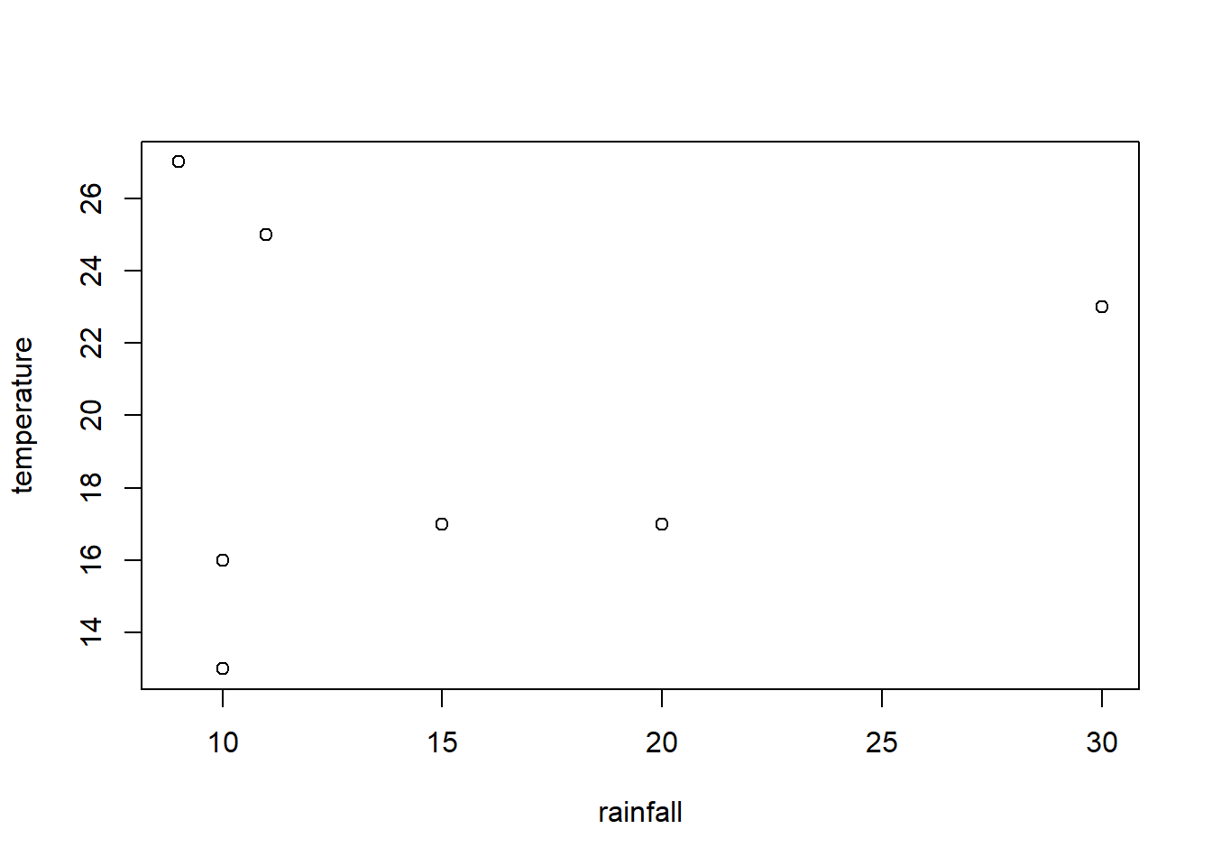
plot(myweather[2:3])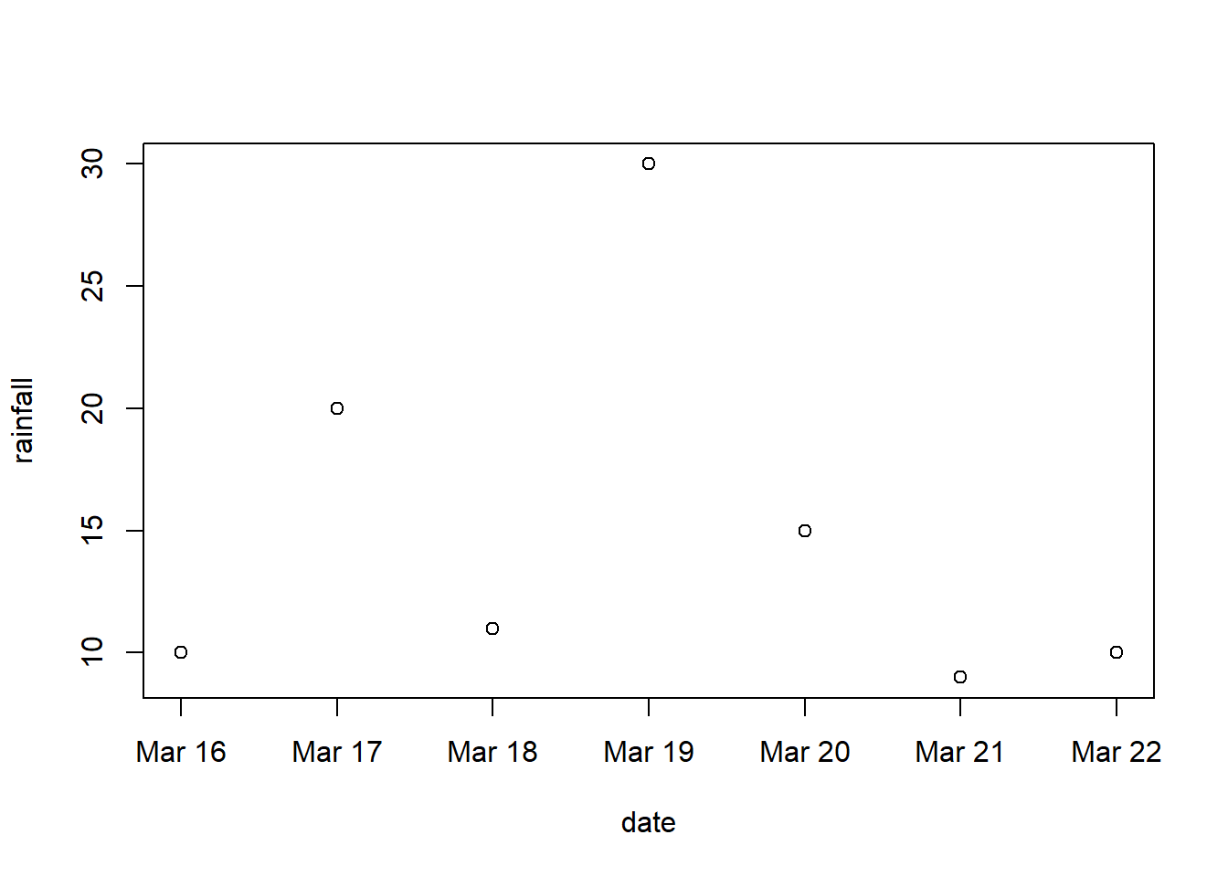
References/Further Reading
- https://www.geeksforgeeks.org/r-language/data-structures-in-r-programming/
- https://www.w3schools.com/r/